Is the NFL's Home-Field Advantage Over?

Introduction

Home-field advantage (HFA) has been documented in many sports, and much speculation has covered the potential causal mechanisms (referee bias, travel times, crowd reactions, etc.). In the NFL, historically, playing at home has offered about a three point advantage in the point differential, the equivalent of a field goal. However, with COVID-19 imposed restrictions, many home games were conducted without fans, and the home team's advantage nearly disappeared. Home teams won 127 of 253 games (50.2%),¹ scoring on average only 0.01 more points than their opponents as opposed to the typical 3.00.

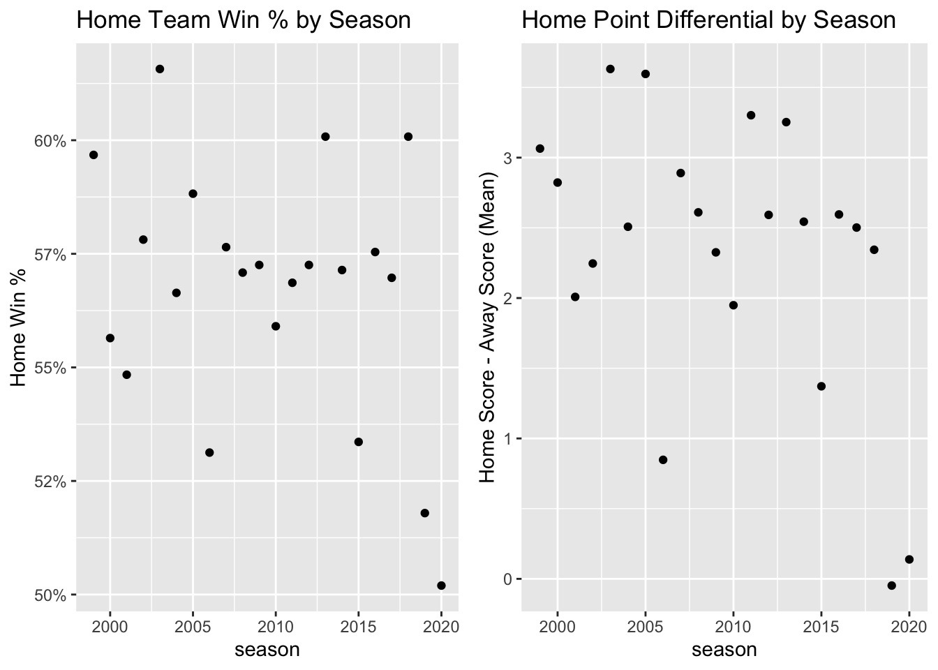
I began this project to see if I could plausibly measure the home-field advantage season-by-season to see just how unusual 2020 was. Indeed, the raw statistics are historic lows for the NFL. 2020 saw the third lowest home point differential (total points scored by home teams minus total points scored by away teams) and the 4th lowest home win percentage since 1966. When examining past seasons, another year jumps out. Just last year in the 2019 season, home teams were outscored by away teams for the first time since 1968. The plots below show the win rates and point differentials for the past 21 regular seasons with games at neutral fields, e.g. international games, removed.

The above are essentially just averages without controlling for team strength. Maybe 2020 and 2019 had unusual schedules that consistently placed lopsided match-ups with the favorite at home. Maybe teams with big home-field advantages and played strong opponents in 2020 and 2019. The rest of this post will investigate whether these two concerns to determine whether the results change when accounting for team strength and heterogeneity in home-field advantage across teams.

Adjusting for team strength

In this section, I will specify a model for measuring home-field advantage while accounting for team strength and analyze home-field advantage over time, both in terms of points and win probability. I will focus primarily on the home team point differential, home team points minus away team points, for each game. This outcome captures what most people care about, the winner and loser, and contains more information than just modeling wins and losses directly. A team that consistently wins by 14 points is probably better than a team that wins by only 7. Using points also avoids having to deal with ties or 16-0 and 0-16 seasons, which pose some technical difficulties that I will explain later.

The model that I will use for point differential is \(Y_{hag} = \alpha_0 + \mu_h - \mu_a + \epsilon_{hag}\) with \(\epsilon_{hag} \sim N(0,\sigma^2)\). \(Y_{hag}\) is the score of home team \(h\) minus the score of away team \(a\) in game \(g\). \(Y_{hag}\) is \(\alpha_0 + \mu_h - \mu_a\) plus some noise, where \(\alpha_0\) captures the home team's scoring advantage, \(\mu_h\) measures the home team's strength and \(\mu_a\) the away team's strength. The model has some nice interpretations of the parameters. \(\alpha_0\) is the expected point differential when two equally skilled teams play. \(\mu_h - \mu_a\) is the expected number of points \(h\) will win or lose by when playing \(a\) on a neutral field. Note that this interpretation is only for the difference in team strength. Each game outcome only provides insight on the relative strength of the teams, so the values of \(\mu_h\) and \(\mu_a\) are not identified, only the differences.² One could, of course, model home points and away points, with separate offensive and defensive HFAs. However, modeling positive, bivariate outcomes gets much more complicated and the primary question of measuring total home-field advantage would ultimately result in estimating a quantity very similar to \(\alpha_0\).

I will also look at simple wins and losses rather than scores to measure home-field advantage. In this case, let the outcome \(W_{hag}\) be a binary variable, 1 for if the home team wins and 0 otherwise. Let \(p_{hag} = P(W_{hag} = 1)\), the probability of a home team win. The model is \(logit(p) = log\left(\frac{p}{1-p}\right) = \alpha_0 + \mu_h - \mu_a\), where \(logit(p)\) refers to the log-odds of the home team winning. The same sort of interpretation applies, just with some slight transformations to account for the fact that the parameters can be any real number while \(p_{hag}\) needs to be between 0 and 1. \(e^{\alpha_0}\) is the odds of the home team winning given equal skill. \(e^{\mu_h - \mu_a}\) is the odds that team \(h\) beats team \(a\) on a neutral field. Note the same identification problem arises in the scale of \(\mu_i\).³

Both models might not look it, but they are actually linear models (or generalized linear for win probabilities) that can be estimated with standard regression packages, just with a clever design matrix. To address the identifiability issues, I enforce a constraint that \(\sum_i \mu_i = 0\). Both models, points and wins, are essentially extensions of the Bradley-Terry model for paired comparisons. See the next section (Implementation Details) for said implementation details. Data, along with team logos and colors used later, were collected from the nflfastR package by Sebastian Carl and Ben Baldwin.

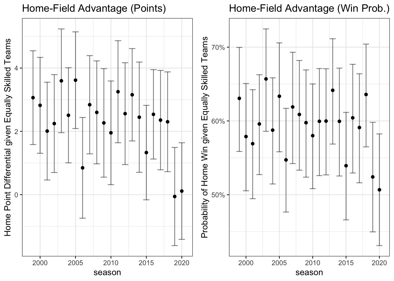
The left panel shows the estimated expected points advantage for the home teams in each season given an opponent of equal strength. The error bars show the 95% confidence intervals. For all but two seasons prior to 2019, we can reject the null that the home-field points advantage is 0. 2019 and 2020 have estimated home-field advantages of -0.075 and 0.114 respectively. Failing to reject the null is of course different from concluding the null is true, but it would be quite challenging to get point estimates closer to zero than what we observe.

In terms of home win probabilities, the results are similar. When two equally skilled teams play, prior to 2019, the home team has an about 60% chance to win. In 2019 and 2020, the confidence intervals exclude 60% for the first time and the home team only had about a 52% and 51% chance of winning, both statistically indistinguishable from a 50-50 chance.

Implementation Details

If you just want to know which teams have the biggest home-field advantages, go ahead and skip to the next section. I assume if you are still here that you have familiarity with multivariate regression and using statistical packages to implement them. I found estimating the previous section's model non-trivial, interesting, and a useful learning experience for dealing with complicated contrasts in OLS and GLM scenarios, so I thought it could help others to document it here.

Here I will describe how I actually implemented the models, focusing on the points model but both are essentially the same. The statement \(Y_{hag} \sim N(\alpha_0 + \mu_h - \mu_a,\sigma^2)\) nicely expresses the model, but it does not look like a standard linear model of the form \(Y = \beta_0 + x_1 \beta_1 + \epsilon\) that most statistical packages request, mostly because of the minus sign and the fact that teams switch sides, playing both home and away games. To use standard estimation tools, essentially, for each game \(g\), we need to come up with a vector of variables \(\mathbf{x}_g\) such that estimated coefficients \(\mathbf{\beta}\) simplify to: \(\mathbf{\beta}^T \mathbf{x}_g = \beta_1 x_{g1} + \beta_2 x_{g2} + \ldots = \alpha_0 + \mu_h - \mu_a\).

Getting \(\alpha_0\) is easy, make \(x_{g1} = 1\) for every game and we get the intercept. Most stats packages don't actually require you to specify the intercept because it is usually not interpretable, but it is our main variable of interest here. Then, for each team \(i\) let \(z_{gi} = 1\) if team \(i\) is the home team in game \(g\), \(-1\) if \(i\) is the away team, and 0 otherwise. If we stack these \(z\) variables together, \(\mu_1 z_{g1} + \mu_2 z_{g2} + \ldots + \mu_{32} z_{g32} = \mu_h - \mu_a\). But we aren't quite done, as you'll notice I've called these variables \(z\) and not the \(x\) that we are interested in. If you try to estimate an intercept plus 32 (one for each NFL team) strength variables, \(z_{32}\) won't estimate. That's because if you add up \(z_1\) through \(z_{31}\) then multiply by -1, you'll get \(z_{32}\) (proof left as an exercise for the reader). This is essentially the identification problem coming back up. Just dropping one of the team strength variables doesn't quite work because the intercept becomes the expected point differential of whatever team was dropped playing at home against a team of strength 0. The dropping uses the identification constraint \(\mu_{32} = 0\) and treats team 32 as the "baseline" team.

The constraint we really want is not for one of the team strength variables to be zero, but rather for them to sum to zero. There is no nice way to tell the software this information because the home and away team information is stored in two different columns of the dataset. So, we have to do it ourselves. In terms of the coefficients, we know \(\sum_{i=1}^{32} \mu_i = 0\) so we can write \(\sum_{i=1}^{31} = -\mu_{32}\). Thus, we can express the regression equation as:

And here we have the final result! Set the variables \(x_{1} = 1\) for the intercept and \(x_{i+1} = z_i - z_{32}\) for \(i\) in 1 to 31 (number of teams \(-1\)), and you have the full equation. We've used the desired constraint to augment the trinary team indicator variables such that the intercept directly measures our quantity of interest. To get the team strength estimates, \(\mu_i\) is the regression coefficient on \(z_i-z_{32}\) and \(\mu_{32}\) is the opposite of the sum of the other \(\mu_i\) terms (ensuring they all sum to zero). Thinking about uncertainty in the estimates of \(\mu_i\) terms is hard because they are all related to each other, if one is an overestimate another must be an underestimate. Dealing with those is outside of the scope of this post, but I may return to it later.

Home-Field Advantage by Team

Finally, I'll look at home-field advantage by team. I'll just do this for the points model because the aforementioned issues with 16-0 and 0-16 seasons get even more common when a home undefeated or win-less season comes up. The extension to the model is simple, I just add a sub script: \(Y_{hag} \sim N(\alpha_h + \mu_h - \mu_a,\sigma^2)\). Now I've written \(\alpha_h\) not \(\alpha_0\) to note that the home-field advantage is home team specific. Estimating this parameter is, however, a bit trickier. In the last model, \(\alpha_0\) was informed directly by all 256 games in a season. Each \(\alpha_h\) is informed by only 8. We can use a similar implementation as above to get a best-guess of each parameter (the maximum likelihood estimate), but those estimates will be quite noisy. Consequently, I will put my Bayesian hat back on and use a hierarchical model for the home team advantage terms: \(\alpha_h \sim N(\alpha_0,\sigma_\alpha^2)\). I assume that the \(\alpha_h\) terms all are drawn from a common distribution. This shrinks the estimates each season towards the "typical" home-field advantage and gives some slight regularization so we done make too extreme estimates given limited data. The model is implemented in stan, and you can find the code over on my GitHub page here.

From the model, I recover posterior beliefs about \(\alpha_0\), the home-field advantage of a typical team in each season, and each \(\alpha_h\), the home-field advantage for team \(h\) in a season. Another important (and new) variable is \(\sigma_{\alpha}\). This is the standard deviation of home-field advantage across teams in a given season. Standard deviations are easy to interpret uncertainty measures: about 50% of the actual \(\alpha_h\) values will be in the interval \(\alpha_0\pm\sigma_\alpha\) and nearly all of the values will be within \(\alpha_0\pm 2\sigma_\alpha\) (about 1 or 2 \(\alpha_h\) values will fall outside of that interval each season). The figure below shows those results.

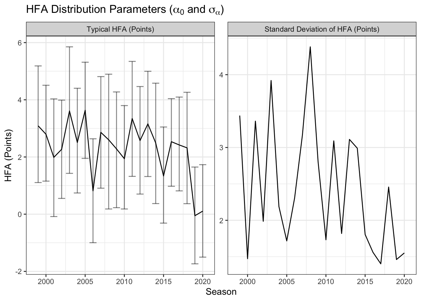
The Typical HFA measures much an average team would be favored at home when playing an equally skilled opponent. These results track with the above results assuming a constant home-field advantage across teams, but for some years the error bars have gotten wider. Certain years, such as 2003 and 2008, had much more variable home-field advantages, which will increase uncertainty in the behavior of an average team. 2008 had most estimates ranging from the home team being favored by about 6 points to being two point underdogs. The next two plots break out the estimates by team. The top panel shows every team and the bottom just the largest and smallest home-field advantages.

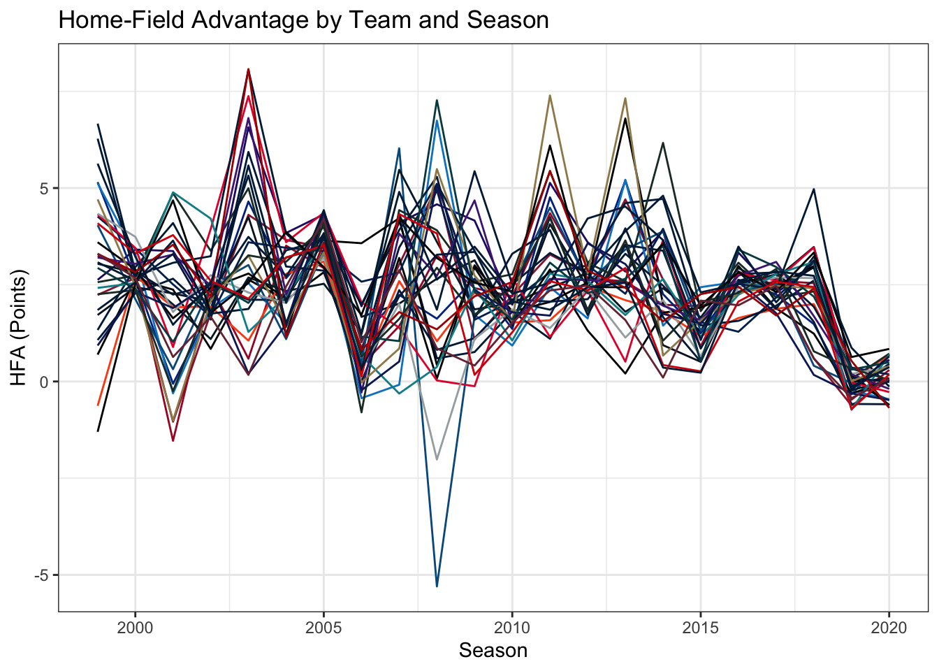
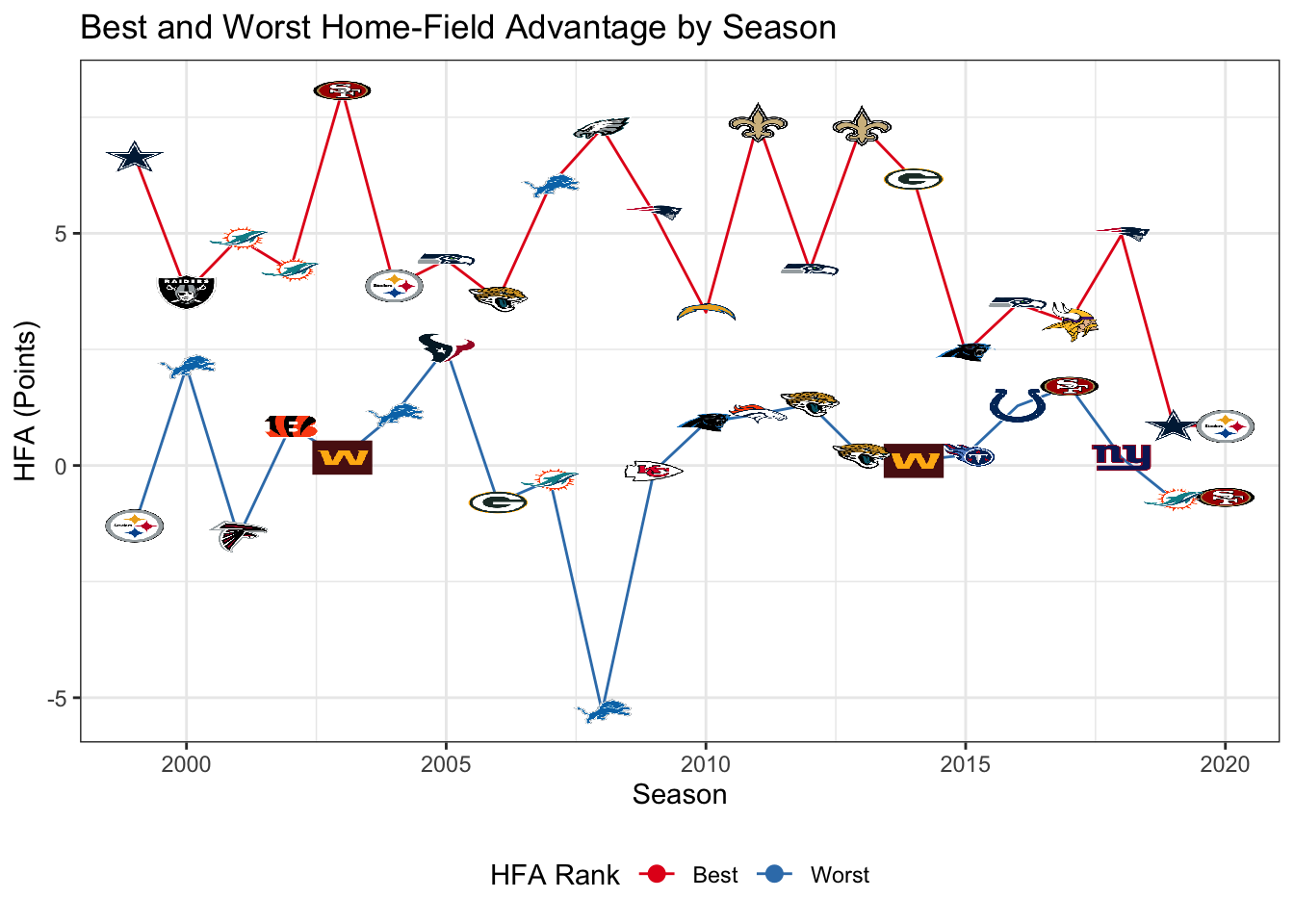
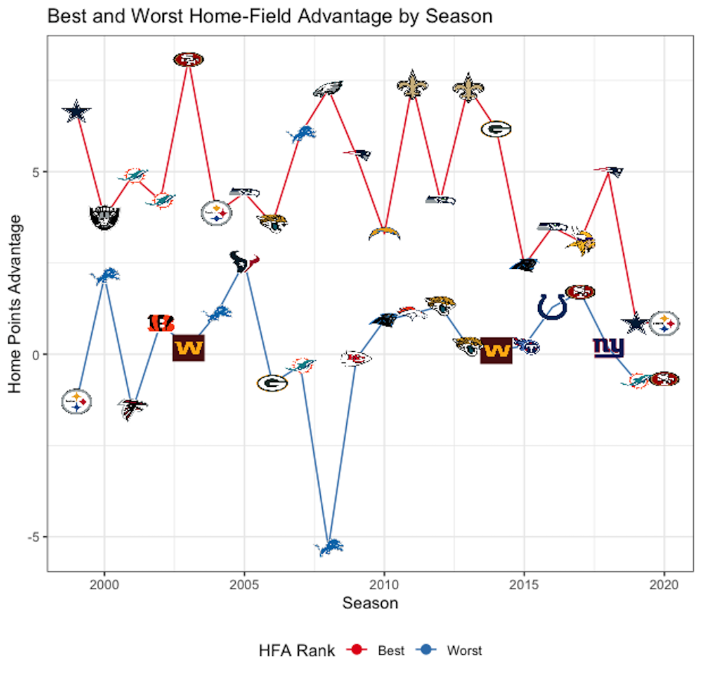
The top plot shows the wide range of home advantages even within a single year, with lines connecting each team's estimate. Starting around 2015, that variability drops off and teams all start to look very similar to each other. Most of the time, the worst home-field advantage is about 0. The outlier in 2008 was the Detroit Lions, who were expected to lose by 5 points at home when playing that they would tie on a neutral field. This was of course the season the Lions went 0-16, losing home games by a significantly larger margin than away games. The bottom plot just picks out the best and worst teams. There is significant turnover year-to-year in the NFL and that pattern continues into home-field advantage. The year prior to the Lions' historically bad year, they had the largest home-field advantage. The 9ers, Dolphins, Jaguars, Panthers, and Steelers also had the smallest and largest home-field advantages in different years, although none of them managed it in consecutive years. To try and review all teams, the table below reports the average and standard deviation of \(\alpha_h\) across all seasons for each team.

	Team	HFA (Mean)	HFA (SD)
	BAL	3.08	1.57
	GB	2.93	1.71
	NE	2.90	1.60
	SEA	2.79	1.47
	PIT	2.62	1.50
	IND	2.59	1.19
	DAL	2.59	1.62
	MIN	2.58	1.59
	LA	2.47	1.87
	SF	2.47	1.76
	NO	2.47	2.19
	PHI	2.38	1.49
	BUF	2.38	1.55
	LAC	2.36	1.44
	DEN	2.34	1.53
	KC	2.32	1.90
	TEN	2.30	1.53
	HOU	2.27	1.17
	CHI	2.25	1.25
	ARI	2.23	1.64
	TB	2.16	1.50
	JAX	2.14	1.26
	CAR	2.12	1.91
	NYJ	2.07	1.25
	ATL	2.02	1.39
	MIA	2.02	1.40
	CIN	1.96	1.52
	DET	1.92	2.28
	LV	1.79	1.37
	NYG	1.75	1.47
	CLE	1.64	0.94
	WAS	1.59	1.21

The Ravens, Packers, Patriots, and Seahawks have the largest average home-field advantages at around 3 to 2.75 point favorites at home. The Lion were only the 5th lowest on average, despite their 2008 results. Washington, the Browns, and the Giants are the three worst home teams. The Jets, who play at the same home stadium as the Giants, are about 2 points better at home than away while the Giants are 1.76 points better. Surprisingly, each team has basically the same standard deviation of home-field advantage at around 2.5 points.

Conclusion

I set out to try and see if the evaporation of home-field advantage in 2020 looked different enough from previous years to claim that the COVID-19 fan and travel restrictions might be a cause of the decline. I found that, yes, home-field advantage was extremely small to non-existent in 2020, but that drop also happened last year in 2019. A few articles discussed it in 2019, but the lack of home-field advantage was discussed much more this year in the context of the global pandemic. However, I don't think the pandemic can be blamed. In recent years, home-field advantage has been very similar across teams, and it dropped to essentially zero last year before the pandemic. Certainly my model could be improved, maybe week 17 games where starters are resting should be dropped, maybe garbage time scores should be removed too, and certainly team strength varies over the course of a season. But I suspect even with more robustness checks and sophisticated tools, the result will remain the same. Other good work on home-field advantage using different methods came to essentially the same conclusions.⁴ The home-field advantage disappeared last year, before anyone had heard of COVID-19.